Solved Assignment course code 4485

فری حل شدہ اسائنمنٹس

BS|Bed Solved Assignment spring 2023

Course: Introduction to Statistics 4485

Semester: Spring, 2023

Level: BS

ASSIGNMENT No. 1

Q. 1 (a) Understanding Statistics and Its Chief Characteristics

Introduction

Statistics is a branch of mathematics that deals with the collection, analysis, interpretation, presentation, and organization of data. It plays a vital role in various fields by providing valuable insights and aiding decision-making processes. In this section, we will delve into the definition of statistics and explore its chief characteristics.

1. Definition of Statistics

Statistics is the science of gathering, analyzing, interpreting, presenting, and organizing data. It involves the use of mathematical principles and techniques to make sense of large datasets and draw meaningful conclusions from them. Statistics allows us to understand trends, patterns, and relationships within the data, thereby enabling us to make informed decisions.

2. Chief Characteristics of Statistics

1. Data-Centric: Statistics revolves around data. It relies on the collection of accurate and relevant data to draw objective conclusions.
2. Objective Approach: It follows an objective approach, emphasizing empirical evidence and avoiding biases or opinions. Statistical analyses are based on measurable evidence, making them reliable and impartial.
3. Quantitative Analysis: Statistics involves the use of numerical data and quantitative techniques for analysis. This allows for precise measurement and comparison of different variables.
4. Generalization: Statistics allows us to make generalizations about a population based on a sample. By studying a representative subset, we can draw conclusions that apply to the entire population.
5. Predictive Insights: One of the chief characteristics of statistics is its ability to provide predictive insights. By analyzing historical data, statisticians can forecast future trends and outcomes.
6. Measure of Variability: Statistics provides measures of variability, such as variance and standard deviation, to understand the spread of data. This helps in assessing the consistency and reliability of the data.
7. Sampling Techniques: Statistics uses various sampling methods to draw conclusions from a subset of the population. These techniques ensure that the sample is representative and reduces the cost and time required for data collection.
8. Interdisciplinary Nature: Statistics is used in diverse fields such as economics, biology, sociology, psychology, and more. Its applicability extends to almost every domain where data analysis is essential.

Q. 1 (b) The Importance of Statistics in Different Fields

1. Economics

Statistics is of immense significance in economics:

• Market Analysis: Statistics helps in analyzing market trends, consumer behavior, and demand-supply patterns. It assists businesses in making informed decisions regarding pricing and production.
• GDP and Economic Growth: Statistical data is used to calculate and analyze the Gross Domestic Product (GDP) and overall economic growth of a country. It provides insights into the economic health of a nation.
• Inflation and Unemployment: Statistics measures inflation rates and unemployment levels, which are crucial indicators of an economy’s performance.

2. Medicine and Healthcare

In the medical field, statistics is indispensable:

• Clinical Trials: Statistics is used to design and analyze clinical trials, evaluating the effectiveness of new drugs or treatments. It helps researchers draw conclusions about the efficacy and safety of medical interventions.
• Epidemiology: Statistics aids in studying the distribution and determinants of diseases in populations. It plays a crucial role in understanding the prevalence and risk factors associated with various illnesses.
• Public Health Policies: Statistical data supports the formulation of public health policies and interventions. It helps in identifying health trends and addressing public health challenges effectively.

3. Education

In the field of education, statistics is highly valuable:

• Assessment and Evaluation: Statistics helps in assessing and evaluating student performance. It enables educators to gauge the effectiveness of teaching methods and educational programs.
• Research Studies: Statistics aids in conducting research studies and analyzing educational data. It facilitates evidence-based decision-making in educational institutions.
• Resource Allocation: Statistical analysis assists in allocating educational resources effectively. It allows educational planners to optimize resource distribution based on data-driven insights.

4. Social Sciences

Statistics is essential for research and analysis in social sciences:

• Sociological Studies: Statistics aids in studying social trends, behaviors, and patterns. It enables sociologists to draw meaningful conclusions about human behavior and societal changes.
• Opinion Polls: Statistics is used to conduct surveys and opinion polls to understand public opinions on various issues. It helps in gauging public sentiment and preferences.
• Demographics: Statistics plays a crucial role in analyzing population demographics and changes. It provides valuable data on population size, age distribution, and migration patterns.

5. Business and Marketing

In the business world, statistics is instrumental:

• Market Research: Statistics aids in conducting market research and analyzing consumer preferences. It helps businesses understand their target audience and tailor their products or services accordingly.
• Financial Analysis: Statistical tools are used to analyze financial data and performance. It assists businesses in making financial forecasts and assessing their financial health.
• Sales Forecasting: Statistics helps in predicting sales and demand for products or services. It allows businesses to plan their inventory and production accordingly.

6. Environmental Science

In environmental science, statistics is of utmost importance:

• Climate Data Analysis: Statistics is used to analyze climate data and study climate patterns. It helps in understanding climate change and its impact on the environment.
• Environmental Impact Assessment: Statistics aids in assessing the environmental impact of various activities, such as construction projects or industrial processes. It assists in identifying potential environmental risks and developing mitigation strategies.
• Biodiversity Studies: Statistics is used to study and monitor biodiversity changes in ecosystems. It helps in assessing the health and stability of ecological systems.

---

Q. 2 (a) Understanding “Classification” and “Tabulation” – Main Steps and Concepts

2. Main Steps in Tabulation (Continued)

• Calculation of Percentages: Calculate percentages to represent the contribution of each category to the whole. Percentages help in comparing the relative significance of different categories in the dataset.
• Formatting the Table: Organize the table with appropriate formatting, including clear headings, proper alignment, and consistent font sizes. A well-formatted table enhances the readability and comprehension of the data.

3. Captions, Stubs, Title, and Prefatory Notes

• Captions: Captions are short descriptions or titles that identify the content of the columns in a table. They serve as labels for the data presented in each column.
• Stubs: Stubs are the labels or headings given to the rows of a table. They provide information about the categories being classified and facilitate easy referencing.
• Title: The title of the table provides a clear description of the data presented. It summarizes the main purpose or findings of the table.
• Prefatory Notes: Prefatory notes are additional explanatory statements or remarks about the table’s content. They can include clarifications, definitions, or any other relevant details to help readers better understand the data.

Q. 2 (b) Explaining the Method of Constructing Histograms with Unequal Class Intervals

Histograms are graphical representations of data that use bars to display the frequency distribution of continuous variables. When dealing with unequal class intervals, the construction of histograms requires special consideration to ensure accurate representation. The steps for constructing histograms with unequal class intervals are as follows:

1. Group the Data: Group the data into intervals that are appropriate for representation. Unlike histograms with equal class intervals, where the width of each interval is the same, histograms with unequal class intervals have varying widths.
2. Calculate Frequency Density: Instead of directly plotting frequencies, calculate frequency density for each interval. Frequency density is the ratio of frequency to the width of the interval. It is calculated by dividing the frequency of each interval by the interval’s width.
3. Plot the Histogram: On a graph, represent each interval’s frequency density by the area of the rectangle formed by the interval’s width and height (frequency density). This accounts for the varying widths of the intervals and ensures that the area of each rectangle accurately reflects the frequency of that interval.
4. Label Axes and Title: Label the horizontal and vertical axes of the graph to represent the intervals and frequencies, respectively. Provide a descriptive title for the histogram to convey the nature of the data being presented.

Histograms with unequal class intervals allow for a more precise representation of the data, especially when the range of values is large or the data is unevenly distributed.

Q. 3 (a) Different Measures of Central Tendency and Their Computation

Measures of central tendency are statistical values that indicate the central or average value in a dataset. There are three main measures of central tendency:

1. Mean: The mean, often referred to as the average, is calculated by summing up all the values in the dataset and dividing by the total number of data points. The formula for calculating the mean (μ) is:

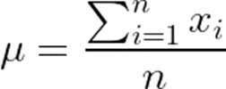
where xi​ represents each data point and n is the total number of data points.

• Median: The median is the middle value of the dataset when it is arranged in ascending or descending order. To find the median, the data must first be sorted. For datasets with an odd number of data points, the median is the value at the exact center of the ordered dataset. For datasets with an even number of data points, the median is the average of the two middle values.
• Mode: The mode is the value that appears most frequently in the dataset. It represents the data point with the highest frequency. A dataset may have one mode (unimodal) or multiple modes (multimodal).

Computation of Mean and Median from the Given Distribution

The given distribution of kilowatt-hours of electricity used in one month by 75 residential consumers in a certain locality of Islamabad is as follows:

Consumption in kWh	5-24	25-44	45-64	65-84	154-162	85-104	105-124
No. of consumers	3	5	9	12	5	4	2

To estimate the mean and median, we need to find the midpoint of each interval and calculate the estimated value.

Estimating the Mean

The midpoint of each interval can be calculated by taking the average of the lower and upper limits of the interval. The estimated value (X) for each interval is:

• For the first interval (5-24): X = (5 + 24) / 2 = 14.5
• For the second interval (25-44): X = (25 + 44) / 2 = 34.5
• For the third interval (45-64): X = (45 + 64) / 2 = 54.5
• For the fourth interval (65-84): X = (65 + 84) / 2 = 74.5
• For the fifth interval (154-162): X = (154 + 162) / 2 = 158
• For the sixth interval (85-104): X = (85 + 104) / 2 = 94.5
• For the seventh interval (105-124): X = (105 + 124) / 2 = 114.5

Next, we multiply each estimated value (X) by the corresponding frequency (f) and sum them up:

Mean (μ) = (3 * 14.5) + (5 * 34.5) + (9 * 54.5) + (12 * 74.5) + (5 * 158) + (4 * 94.5) + (2 * 114.5) = 1231.5

Finally, we divide the sum by the total number of consumers (75) to find the mean:

Mean (μ) = 1231.5 / 75 ≈ 16.42

Estimating the Median

To estimate the median, we need to find the middle value of the dataset when it is arranged in ascending order. We can do this by considering the cumulative frequencies of the intervals.

The cumulative frequencies for each interval are:

• For the first interval (5-24): 3
• For the second interval (25-44): 3 + 5 = 8
• For the third interval (45-64): 8 + 9 = 17
• For the fourth interval (65-84): 17 + 12 = 29
• For the fifth interval (154-162): 29 + 5 = 34
• For the sixth interval (85-104): 34 + 4 = 38
• For the seventh interval (105-124): 38 + 2 = 40

Since the total number of consumers is 75, the median falls in the 38th interval, which is (85-104). The midpoint of this interval is:

X = (85 + 104) / 2 = 94.5

Thus, the estimated median for the given distribution is 94.5 kWh.

Q. 4 (a) The Empirical Relationship between Mean, Median, and Mode

The empirical relationship between the mean, median, and mode depends on the skewness of the data distribution:

1. Symmetric Distribution: In a perfectly symmetric dataset, where the frequency of values is balanced around the center, the mean, median, and mode are equal. This scenario is commonly observed in normal distributions.
2. Positively Skewed Distribution: In a positively skewed distribution, the tail of the data points extends more towards higher values. In such cases, the mean is generally greater than the median and the mode. The mean is pulled in the direction of the long tail by the extreme values, while the median remains closer to the central data points.
3. Negatively Skewed Distribution: In a negatively skewed distribution, the tail of the data points extends more towards lower values. Here, the mean is usually less than the median and the mode. The mean is pulled toward the lower values by the extreme data points, causing it to be lower than the median, which represents the central tendency of the majority of data points.

Q. 4 (b) Calculating Mode from the Given Data

To calculate the mode from the given data, we need to identify the value with the highest frequency. The data is provided as follows:

X	22	24	26	28	30	32	34	36	38	40	42	44
f	3	13	43	102	175	220	204	139	69	25	6	1

The value with the highest frequency is 32, as it appears 220 times in the dataset. Therefore, the mode for this data set is 32.

Q. 5 (a) Criteria of a Suitable Average

A suitable average should possess the following characteristics:

1. Representative: The average should accurately represent the general tendency of the data. It should give a fair idea of the central value around which the data points cluster.
2. Unbiased: The average should not be heavily influenced by extreme values or outliers. It should not be overly affected by rare occurrences that do not reflect the typical pattern of the dataset.
3. Easy to Understand: The average should be easily interpretable and straightforward for non-experts to comprehend. It should provide a clear and concise summary of the data.
4. Easy to Compute: The calculation of the average should be simple and feasible, allowing for efficient and quick determination of the value.
5. Appropriate for Data Type: Different types of data (e.g., numerical, categorical, ordinal) require different types of averages. For instance, the arithmetic mean is suitable for numerical data, while the mode is appropriate for categorical data.

Q. 5 (b) Calculating Geometric Mean and Harmonic Mean from the Given Distribution

The given distribution is as follows:

Classes	4-6	6-8	8-10	10-12	12-14	14-16
f	13	11	182	105	19	7

Calculating the Geometric Mean

The geometric mean is used when dealing with data that has multiplicative relationships. To calculate the geometric mean, follow these steps:

1. Multiply all values together: Multiply the class midpoint of each interval by its corresponding frequency (f).
2. For the first interval (4-6): X1​=5, f1​=13
3. For the second interval (6-8): ​=7, ​=11
4. For the third interval (8-10): ​=9, ​=182
5. For the fourth interval (10-12): X4​=11, ​=105
6. For the fifth interval (12-14): X5​=13, f5​=19
7. For the sixth interval (14-16):X6=15, f6​=7

The product of all values is: P=(5¹³)∗(7¹¹)∗(9¹⁸²)∗(11¹⁰⁵)∗(13¹⁹)∗(15⁷)

• Take the nth root of the product: Calculate the geometric mean (GM) by taking the 1/nth root of the product, where n is the total frequency (sum of all frequencies).

GM = P(1/n)

Sum of all frequencies (n) = 13 + 11 + 182 + 105 + 19 + 7 = 337

GM = P(1/337)

GM ≈ 9.54 (rounded to two decimal places)

The geometric mean of the given distribution is approximately 9.54.

Calculating the Harmonic Mean

The harmonic mean is used when dealing with data that has rates or ratios. To calculate the harmonic mean, follow these steps:

1. Find the reciprocal of each value: Take the reciprocal of each class midpoint.
2. For the first interval (4-6): X1​=5, so the reciprocal R1​=51​
3. For the second interval (6-8): ​=7, so the reciprocal R2​=71​
4. For the third interval (8-10): X3​=9, so the reciprocal R3​=91​
5. For the fourth interval (10-12): X4​=11, so the reciprocal R4​=111​
6. For the fifth interval (12-14): X5​=13, so the reciprocal R5​=131​
7. For the sixth interval (14-16): X6​=15, so the reciprocal R6​=151​
8. Calculate the arithmetic mean of the reciprocals: Add all the reciprocals together and divide by the number of intervals (6 in this case).

Harmonic Mean (HM) = 666R1​+R2​+R3​+R4​+R5​+R6​​

HM = 15+17+19+111+113+1156651​+71​+91​+111​+131​+151​​

HM ≈ 0.1009 (rounded to four decimal places)

The harmonic mean of the given distribution is approximately 0.1009.